First let's clarify what fast Fourier Transform is and why you want to use it. The mathematics is all about frequencies. The Fourier Transform is a method to single out smaller waves in a complex wave. That sounded complex; when you listen to music you hear many different notes from the singer, instruments and so on. As humans we can often hear the guitar on its own but try to single it out with technology in a recording and you run into trouble. Modern technology can do it, thanks to the different incarnations of the basic Fourier equations that were developed through the years. Modern uses of the Fourier series are picture and video compression, GPS and MRI scans. All these makes an approximation of the source and use Fourier series to save memory and get faster results.
The mathematician Jean-Baptiste Joseph Fourier was actually trying to solve the heat equation, to make it possible to calculate how heat propagates in solid matter. What he came up with was far more useful than that, eventhough his methods was later improved to a more formal version. The equations are now used in a wide range of fields.
To single out a specific frequency in a complex signal you can use some calculations, the Fast Fourier Transforms. The mathematical foundation for this takes some practice. Khan Academy is a nice place to learn the math.
When you need to analyse any waves, you can use sine functions to approximate the total wave and get all the separate signals from the mixed wave. Or vice versa, you can make a complex wave from several sine waves. This is the basic idea behind the mathematics.
To understand your Fourier Transforms better, a good practice is to write them yourself. In Scilab you have a simple programming language designed with emphasis on mathematics.
The different tasks you will need Fourier transforms start with finding the coefficients of a transform. The reason is that this is what is used for compression of pictures and many other processes.
When you learn the basics of the series, the first thing that is uses are the coefficients. The equations are like this:

The code to solve them is fairly simple, it begins with a function. This function implements the Fourier Transform in small pieces.
To define a function you use the obvious 'function' construct. Below is a fourier series for a square wave:
y=4*sin(t)/1*%pi + 4*sin(3*t)/3*%pi + 4*sin(5*t)/5*%pi + 4*sin(7*t)/7*%pi
+ 4*sin(9*t)/9*%pi
endfunction
To make the wave even more square, it is an approximation after all, you need to keep increasing the number of terms. When you are looking to recreate a pattern, say a cartoon, you use the Fourier transform in a very similar way. You just need to consider the period as infinite.
Simple right? Well, not without the basic math knowledge. Try a few examples yourself, using scilab.
This example shows the simplest possible signal combination; two signals of different frequency.
//Choose a sample sizeN = 100;
//Set the sequence, this creates the array
n = 0:N-1;
//Create the frequency of the signals
w1 = %pi/4
w2 = %pi/8
//Make the sampled signals
s1 = cos(w1*n);// The first component of the signal
s2 = cos(w2*n);// The second component of the signal
//Combine the two into one signal
//In this case we make a simple clean signal.
f = s1 + s2;
//Here is the resulting signal ready for transform.
figure(0);
plot(f);
//The Fourier transform of this signal should show only the frequency of the components.
F = fft(f);
F_abs = abs(F);
figure(1);
plot(n,F_abs);
figure(2);
plot(F);
Use the above example to practice how the transform works. Make sure you change it to filter in different ways.
A tip is to use the Scilab console to see what the variables contain at each step of the program, this way you can also see that 'F' has an imaginary content. Try to change äfä in another way to get a more correct result.
In industry, the most common use of Fourier Transforms is for analyzing signal. To filter out frequencies out of a noisy signal, you need to start with making, or importing a signal. The following code snippet creates a mixed signal of two frequencies, 50 and 70 hz. In the code you can also see the use of 'grand', this is the scilab call to random. These random values are added to make the signal a bit more noisy, closer to reality.
sample_rate=1000;t = 0:1/sample_rate:0.6;
N=size(t,'*'); //number of samples
s=sin(2*%pi*50*t)+sin(2*%pi*70*t+%pi/4)+grand(1,N,'nor',0,1);
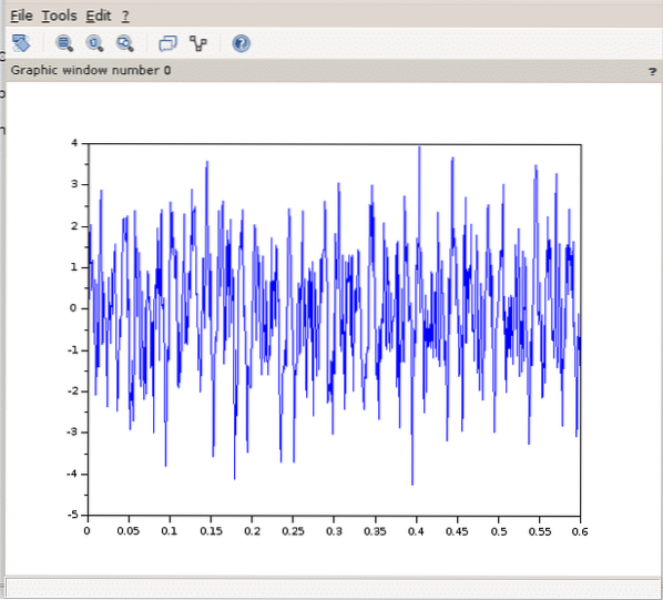
Now, you can plot 's' as a function of 't' and see that the graph looks messy.
>>plot(t,s);
Here, it is time to try out the simplest of fourier transforms, make 'y' the fourier transform of s.
y=fft(s);fft
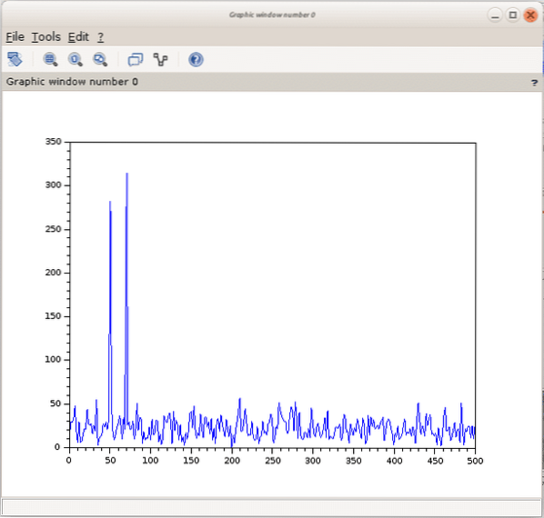
If you plot 'y' as a function of 't', you get a somewhat symmetric pattern ranging from 0 to 0.6. The two spikes are what we are looking for but we are now seeing them in the time domain. What really happened was that the result still contained the imaginary values. To find the two frequencies in the frequency domain, we need some more operationsto find only the real numbers. And then you take the absolute value of the results. The graph clearly points out the original frequencies.
Here is the code:
//s is real so the fft response is conjugate symmetric and we retain only the firstN/2 points
f=sample_rate*(0:(N/2))/N; //associated frequency vector
n=size(f,'*')
clf()
plot(f,absy(1:n)))
This is the most common use of the Fourier transform. Using this system you can find any frequency in a complex, noisy signal. The equations are widely used in many industries today.
The fft2 function of Scilab is the two-dimensional version of fast fourier transformation.
One great way to practice is to pick the DTMF tones, create one button press and have scilab figure out the correct key.
The demos in Scilab itself contains a sound file showcase, study it.
If you want to dig deeper, here are a few links to further reading.
Advanced literature:
https://cnx.org/contents/[email protected]/Implementing-FFTs-in-Practice#uid8
Wolfram…
http://demonstrations.wolfram.com/ComplexAndRealPlanesOfDiscreteFourierTransforms/
Implementing in other languages:
https://www.nayuki.io/page/how-to-implement-the-discrete-fourier-transform
To get the right feel for the subject:
https://betterexplained.com/articles/an-interactive-guide-to-the-fourier-transform/